
PyODPS is the Python SDK of MaxCompute. It supports basic actions on MaxCompute objects and the DataFrame framework for ease of data analysis on MaxCompute. For more information, see the GitHub project and the PyODPS Documentation that describes all interfaces and classes.
-
Developers are invited to participate in the ecological development of PyODPS. For more information, see GitHub document.
-
Developers can also submit the issue and merge request to accelerate PyODPS eco-growth. For more information, see code
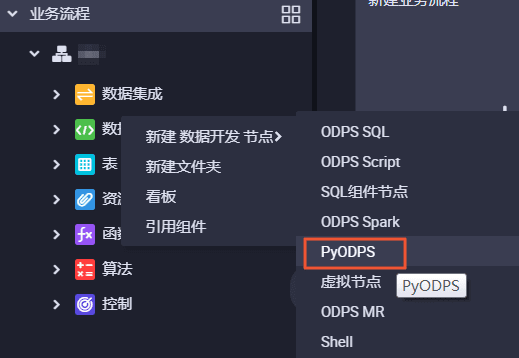
Installation PyODPS
PyODPS supports Python 2.6 and later versions. After installing PIP in the system, you only need to run pip install pyodps. The related dependencies of PyODPS are automatically installed.
Quick start
Log on using your Alibaba Cloud primary account to initialize a MaxCompute entry, as shown in the following code:
from odps import ODPS
odps = ODPS('**your-access-id**', '**your-secret-access-key**', '**your-default-project**',
            endpoint='**your-end-point**')
After completing initialization, you can operate tables, resources, and functions.
Project
A project is the basic unit of operation in MaxCompute, similar to a database.
Call get_project to obtain a project, as shown in the following code:
project = odps.get_project('my_project') # Obtain a project.
project = odps.get_project() # Obtain the default project.
Note
- If parameters are not input, use the default project.
-
You can call
exist_projectto check whether the project exists. -
A table is a data storage unit of MaxCompute.
Table action
Call list_tables to list all tables in the project, as shown in the following code:
for table in odps.list_tables():
    # Process each table
Call exist_table to check whether the table exists and call get_table to obtain the table.
t = odps.get_table('dual')
t.schema
odps.Schema {
  c_int_a                 bigint
  c_int_b bigint
  c_double_a double
  c_double_b double
  c_string_a string
  c_string_b string
  c_bool_a boolean
  c_bool_b boolean
  c_datetime_a datetime
  c_datetime_b datetime
}
t.lifecycle
-1
print(t.creation_time)
2014-05-15 14:58:43
t.is_virtual_view
False
t.size
1408
t.schema.columns
[<column c_int_a, type bigint>,
 <column c_int_b, type bigint>,
 <column c_double_a, type double>,
 <column c_double_b, type double>,
 <column c_string_a, type string>,
 <column c_string_b, type string>,
 <column c_bool_a, type boolean>,
 <column c_bool_b, type boolean>,
 <column c_datetime_a, type datetime>,
 <column c_datetime_b, type datetime>]
Create schema for a table
Two initialization methods are as follows:
- Initialize through table columns and optional partitions, as shown in the following code:
from odps.models import Schema, Column, Partition columns = [Column(name='num', type='bigint', comment='the column')] partitions = [Partition(name='pt', type='string', comment='the partition')] schema = Schema(columns=columns, partitions=partitions) schema.columns [<column num, type bigint>, <partition pt, type string>] - Although it is easier to call
Schema.from_listsfor initialization, annotations of columns and partitions cannot be set directly.schema = Schema.from_lists(['num'], ['bigint'], ['pt'], ['string']) schema.columns [<column num, type bigint>, <partition pt, type string>]
Create a table
Use a table schema to create a table, as shown in the following code:
table = odps.create_table('my_new_table', schema)
table = odps.create_table('my_new_table', schema, if_not_exists=True) # Create a table only when no table exists.
table = o.create_table('my_new_table', schema, lifecycle=7) # Set the life cycle.
Use a field name field type string connected by commas (,) to create a table, as shown in the following code:
>>> # Create a non-partition table.
>>> table = o.create_table('my_new_table', 'num bigint, num2 double', if_not_exists=True)
>>> # To create a partition table, you can input (list of table fields, list of partition fields).
>>> table = o.create_table('my_new_table', ('num bigint, num2 double', 'pt string'), if_not_exists=True)
Without related settings, you can use only the BIGINT, DOUBLE, DECIMAL, STRING, DATETIME, BOOLEAN, MAP, and ARRAY types when creating a table.
If your service is on a public cloud, or supports new data types such as TINYINT or STRUCT, you can set options.sql.use_odps2_extension = True to enable the new types, as shown in the following code:
from odps import options
options.sql.use_odps2_extension = True
table = o.create_table('my_new_table', 'cat smallint, content struct<title:varchar(100), body string>')
Obtain table data
Table data can be obtained using three methods:
- Call
headto obtain table data as follows (only the first 10,000 data records or fewer of each table can be obtained):>>> t = odps.get_table('dual') >>> for record in t.head(3): >>> print(record[0]) # Obtain the value at the zero position. >>> print(record['c_double_a']) # Obtain a value through a field. >>> print(record[0: 3]) # Slice action >>> print(record[0]) # Obtain values at multiple positions. >>> print(record['c_int_a', 'c_double_a']) # Obtain values through multiple fields. - Run
open_readeron a table to open a reader to read data. You can use the WITH expression:# Use the with expression. with t.open_reader(partition='pt=test') as reader: count = reader.count for record in reader[5:10] # This action can be performed multiple times until a certain number (indicated by count) of records are read. This statement can be transformed to parallel action. # Process a record. # Do not use the with expression. reader = t.open_reader(partition='pt=test') count = reader.count for record in reader[5:10] # Process a record. - Call the Tunnel API to read table data. The
open_readeraction is encapsulated in the Tunnel API.
Write data
A table object can also perform the open_writer action to open the writer and write data, which is similar to open_reader.
Example:
 # Use the with expression.
 with t.open_writer(partition='pt=test') as writer:
     writer.write(records) # Here, records can be any iteratable records and are written to block 0 by default.

 with t.open_writer(partition='pt=test', blocks=[0, 1]) as writer: # Open two blocks at the same time
     writer.write(0, gen_records(block=0))
     writer.write(1, gen_records(block=1)) # The two write operations can be parallel in multiple threads. Each block is independent.

 # Do not use the WITH expression.
 writer = t.open_writer(partition='pt=test', blocks=[0, 1])
 writer.write(0, gen_records(block=0))
 writer.write(1, gen_records(block=1))
 writer.close() # You must close the writer. Otherwise, the written data may be incomplete.
Similarly, writing data into the table is encapsulated in the Tunnel API.
Delete a table
Delete a table as shown in the following code:
odps.delete_table('my_table_name', if_exists=True) # Delete a table only when the table exists
 t.drop() # The drop function can be directly executed if a table object exists.
Table partitioning
- Basic operations
Traverse all partitions of a table as shown in the following code:
for partition in table.partitions:
    print(partition.name)
 for partition in table.iterate_partitions(spec='pt=test'):
    Traverse list partitions.
Check whether a partition exists as shown in the following code:
table.exist_partition('pt=test,sub=2015')Obtain the partition as shown in the following code:
partition = table.get_partition('pt=test') print(partition.creation_time) 2015-11-18 22:22:27 partition.size 0 - Create a partition
t.create_partition('pt=test', if_not_exists=True) # Create a partition only when no partition exists. - Delete a partition
 t.delete_partition('pt=test', if_exists=True) # Delete a partition only when the partition exists.
 partition.drop() # Directly drop a partition if a partition object exists.
SQL
PyODPS supports MaxCompute SQL query and can directly read the execution results.
- Run the SQL statements
odps.execute_sql('select * from dual') # Run SQL in synchronous mode. Blocking continues until SQL execution is completed. instance = odps.run_sql('select * from dual') # Run the SQL statements in asynchronous mode. instance.wait_for_success() # Blocking continues until SQL execution is completed. - Read the SQL statement execution results
The instance that runs the SQL statements can directly perform the
open_readeraction. In one scenario, the SQL statements return structured data, as follows:with odps.execute_sql('select * from dual').open_reader() as reader: for record in reader: # Process each record.
In the second scenario, the actions that may be performed by SQL, such as desc, obtain the raw SQL execution result through the reader.raw attribute, as follows:
with odps.execute_sql('desc dual').open_reader() as reader:
    print(reader.raw)
Resources
Resources commonly apply to UDF and MapReduce on MaxCompute.
You can use list_resources to list all resources and use exist_resource to check whether a resource exists. You can call delete_resource to delete resources or directly call the drop method for a resource object.
PyODPS mainly supports two resource types: file resources and table resources.
- File resources
File resources include the basic
filetype, andpy,jar, andarchive.Note In DataWorks, file resources in the py format must be uploaded as files.Create a file resource
Create a file resource by specifying the resource name, file type, and a file-like object (or a string object), as shown in the following example:
resource = odps.create_resource('test_file_resource', 'file', file_obj=open('/to/path/file')) # Use a file-like object.
resource = odps.create_resource('test_py_resource', 'py', file_obj='import this') # Use a string.
Read and modify a file resource
You can call theopenmethod for a file resource or callopen_resourceat the MaxCompute entry to open a file resource. The opened object is a file-like object. Similar to theopenmethod built in Python, file resources also support the open mode.Example:
 with resource.open('r') as fp: # Open a resource in read mode.
    content = fp.read() # Read all content.
    fp.seek(0) # Return to the start of the resource.
    lines = fp.readlines() # Read multiple lines.
    fp.write('Hello World') # Error. Resources cannot be written in read mode.
with odps.open_resource('test_file_resource', mode='r+') as fp: # Enable read/write mode.
    fp.read()
    fp.tell() # Current position
    fp.seek(10)
    fp.truncate() # Truncate the following content.
    fp.writelines(['Hello\n', 'World\n']) # Write multiple lines.
    fp.write('Hello World')
    fp.flush() # Manual call submits the update to MaxCompute.
The following open modes are supported:
r: Read mode. The file can be opened but cannot be written.w: Write mode. The file can be written but cannot be read. Note that file content is cleared first if the file is opened in write mode.a: Append mode. Content can be added to the end of the file.r+: Read/write mode. You can read and write any content.w+: Similar tor+, but file content is cleared first.a+: Similar tor+, but content can be added at the end of the file only during writing.
In PyODPS, file resources can be opened in a binary mode. For example, some compressed files must be opened in binary mode.
rbindicates opening a file in binary read mode, andr+bindicates opening a file in binary read/write mode. - Table resources
Create a table resource
>>> odps.create_resource('test_table_resource', 'table', table_name='my_table', partition='pt=test')Update a table resource
>>> table_resource = odps.get_resource('test_table_resource')
>>> table_resource.update(partition='pt=test2', project_name='my_project2')
DataFrame
PyODPS offers DataFrame API, which provides interfaces similar to pandas, but can fully utilize computing capability of MaxCompute. For more information, see DataFrame.
The following is an example of DataFrame:
o = ODPS('**your-access-id**', '**your-secret-access-key**',
             project='**your-project**', endpoint='**your-end-point**'))
Here, movielens 100K is used as an example. Assume that three tables already exist, namely, pyodps_ml_100k_movies (movie-related data), pyodps_ml_100k_users (user-related data), and pyodps_ml_100k_ratings (rating-related data).
You only need to input a Table object to create a DataFrame object. For example:
from odps.df import DataFrameusers = DataFrame(o.get_table('pyodps_ml_100k_users'))View fields of DataFrame and the types of the fields through the dtypes attribute, as shown in the following code:
users.dtypesYou can use the head method to obtain the first N data records for data preview.
Example:
users.head(10)| user_id | age | sex | occupation | zip_code | |
|---|---|---|---|---|---|
| 0 | 1 | 24 | M | technician | 85711 |
| 1 | 2 | 53 | F | other | 94043 |
| 2 | 3 | 23 | M | writer | 32067 |
| 3 | 4 | 24 | M | technician | 43537 |
| 4 | 5 | 33 | F | other | 15213 |
| 5 | 6 | 42 | M | executive | 98101 |
| 6 | 7 | 57 | M | administrator | 91344 |
| 7 | 8 | 36 | M | administrator | 05201 |
| 8 | 9 | 29 | M | student | 01002 |
| 9 | 10 | 53 | M | lawyer | 90703 |
You can add a filter on the fields to view selective fields only.
Example:
users[['user_id', 'age']].head(5)| user_id | age | |
|---|---|---|
| 0 | 1 | 24 |
| 1 | 2 | 53 |
| 2 | 3 | 23 |
| 3 | 4 | 24 |
| 4 | 5 | 33 |
You can also exclude several fields.
Example:
users.exclude('zip_code', 'age').head(5)| user_id | Sex | Occupation | |
|---|---|---|---|
| 0 | 1 | M | Technician |
| 1 | 2 | F | Other |
| 2 | 3 | M | Writer |
| 3 | 4 | M | Technician |
| 4 | 5 | F | Other |
If you want to exclude selective fields, and obtain new columns through computation use the code as shown in the following example:
For example, add the sex_bool attribute and set it to True if sex is Male. Otherwise, set it to False.
Example:
users.select(users.exclude('zip_code', 'sex'), sex_bool=users.sex == 'M').head(5)| user_id | Age | Occupation | sex_bool | |
|---|---|---|---|---|
| 0 | 1 | 24 | Technician | True |
| 1 | 2 | 53 | Other | False |
| 2 | 3 | 23 | Writer | True |
| 3 | 4 | 24 | Technician | True |
| 4 | 5 | 33 | Other | False |
Obtain the number of persons between 20 and 25 age group, as shown in the following code:
users.age.between(20, 25).count().rename('count')
943
Obtain the numbers of male and female users, as shown in the following code:
users.groupby(users.sex).count()| Sex | Count | |
|---|---|---|
| 0 | Female | 273 |
| 1 | Male | 670 |
To divide users by job, obtain the first 10 jobs that have the largest population, and sort the jobs in the descending order of population.
Example:
>>> df = users.groupby('occupation').agg(count=users['occupation'].count())
>>> df.sort(df['count'], ascending=False)[:10]| Occupation | Count | |
|---|---|---|
| 0 | Student | 196 |
| 1 | Other | 105 |
| 2 | Educator | 95 |
| 3 | Administrator | 79 |
| 4 | Engineer | 67 |
| 5 | Programmer | 66 |
| 6 | Librarian | 51 |
| 7 | Writer | 45 |
| 8 | Executive | 32 |
| 9 | Scientist | 31 |
DataFrame APIs provide the value_counts method to quickly achieve the same result. For example:
users.occupation.value_counts()[:10]| Occupation | Count | |
|---|---|---|
| 0 | Student | 196 |
| 1 | Other | 105 |
| 2 | Educator | 95 |
| 3 | Administrator | 79 |
| 4 | Engineer | 67 |
| 5 | Programmer | 66 |
| 6 | Librarian | 51 |
| 7 | Writer | 45 |
| 8 | Executive | 32 |
| 9 | Scientist | 31 |
Show data in a more intuitive graph, as shown in the following code:
%matplotlib inlineUse a horizontal bar chart to visualize data, as shown in the following code:
users['occupation'].value_counts().plot(kind='barh', x='occupation',
ylabel='prefession')
Divide ages into 30 groups and view the histogram of age distribution, as shown in the following code:
users.age.hist(bins=30, title="Distribution of users' ages", xlabel='age', ylabel='count of users')
Use JOIN to join the three tables and save the joined tables as a new table.
Example:
movies = DataFrame(o.get_table('pyodps_ml_100k_movies'))
ratings = DataFrame(o.get_table('pyodps_ml_100k_ratings'))
o.delete_table('pyodps_ml_100k_lens', if_exists=True)
 lens = movies.join(ratings).join(users).persist('pyodps_ml_100k_lens')
 lens.dtypes
odps.Schema {
movie_id int64
title string
release_date string
video_release_date string
imdb_url string
user_id int64
rating int64
unix_timestamp int64
age int64
sex string
occupation string
zip_code string
}Divide the age groups between 0 and 80 into eight groups, as shown in the following code:
 labels = ['0-9', '10-19', '20-29', '30-39', '40-49', '50-59', '60-69', '70-79']
 cut_lens = lens[lens, lens.age.cut(range(0, 81, 10), right=False, labels=labels).rename('age group')]
View the first 10 data records of a single age group in a group, as shown in the following code:
>>> cut_lens['age group', 'age'].distinct()[:10]| Age-group | Age | |
|---|---|---|
| 0 | 0-9 | 7 |
| 1 | 10-19 | 10 |
| 2 | 10-19 | 11 |
| 3 | 10-19 | 13 |
| 4 | 10-19 | 14 |
| 5 | 10-19 | 15 |
| 6 | 10-19 | 16 |
| 7 | 10-19 | 17 |
| 8 | 10-19 | 18 |
| 9 | 10-19 | 19 |
View users’ total rating and average rating of each age group, as shown in the following code:
cut_lens.groupby('age group').agg(cut_lens.rating.count().rename('total rating'), cut_lens.rating.mean().rename('average rating'))| Age-group | Average rating | Total rating | |
|---|---|---|---|
| 0 | 0-9 | 3.767442 | 43 |
| 1 | 10-19 | 3.486126 | 8181 |
| 2 | 20-29 | 3.467333 | 39535 |
| 3 | 30-39 | 3.554444 | 25696 |
| 4 | 40-49 | 3.591772 | 15021 |
| 5 | 50-59 | 3.635800 | 8704 |
| 6 | 60-69 | 3.648875 | 2623 |
| 7 | 70-79 | 3.649746 | 197 |
Configuration
PyODPS provides a series of configuration options, which can be obtained through odps.options. The following lists configurable MaxCompute options:
- General configuration
Option Description Default value end_point MaxCompute Endpoint. None default_project Default Project. None log_view_host LogView host name. None log_view_hours LogView holding time (in hours). 24 local_timezone Used time zone. True indicates local time, and False indicates UTC. The time zone of pytz can also be used. 1 lifecycle Life cycles of all tables. None temp_lifecycle Life cycles of the temporary tables. 1 biz_id User ID. None verbose Whether to print logs. False verbose_log Log receiver. None chunk_size Size of write buffer. 1496 retry_times Request retry times. 4 pool_connections Number of cached connections in the connection pool. 10 pool_maxsize Maximum capacity of the connection pool. 10 connect_timeout Connection time-out. 5 read_timeout Read time-out. 120 completion_size Limit on the number of object complete listing items. 10 notebook_repr_widget Use interactive graphs. True sql.settings MaxCompute SQL runs global hints. None sql.use_odps2_extension Enable MaxCompute 2.0 language extension. False - Data Upload/Download configuration
Option Description Default value tunnel.endpoint Tunnel Endpoint. None tunnel.use_instance_tunnel Use Instance Tunnel to obtain the execution result. True tunnel.limited_instance_tunnel Limit the number of results obtained by Instance Tunnel. True tunnel.string_as_binary Use bytes instead of unicode in the string type. False - DataFrame Configurations
Option Description Default value interactive Whether in an interactive environment. Depend on the detection value df.analyze Whether to enable non-MaxCompute built-in functions. True df.optimize Whether to enable DataFrame overall optimization. True df.optimizes.pp Whether to enable DataFrame predicate push optimization. True df.optimizes.cp Whether to enable DataFrame column tailoring optimization. True df.optimizes.tunnel Whether to enable DataFrame tunnel optimization. True df.quote Whether to use “ to mark fields and table names at the end of MaxCompute SQL. True df.libraries Third-party library (resource name) that is used for DataFrame running. None - PyODPS ML Configurations
Option Description Default value ml.xflow_project Default Xflow project name. algo_public ml.use_model_transfer Whether to use ModelTransfer to obtain the model PMML. True ml.model_volume Volume name used when ModelTransfer is used. pyodps_volume
Summary
In this blog, you’ve got to see a bit more about Alibaba Cloud MaxCompute PyODPS to take advantage of all of the features included in MaxCompute to help kickstart your data processing and analytics workflow.